fftab • fftab

The fftab package provides a tidy interface for Fourier Transform operations by storing Fourier coefficients and their associated frequencies in a tabular format (tibble). This design facilitates the manipulation of spectral data using pipes and functions from the tidyverse.

We’ll demonstrate the package’s capabilities using reproducible examples.

Setup

Load the package and set the random seed:

library(fftab)
set.seed(1234)

The fftab function supports various input types, including numeric and complex vectors, time series objects, and multidimensional arrays.

Vector Input

A simple example is the FFT of a numeric vector:

v <- rnorm(8)

v_fft <- fftab(v)

print(v_fft)
#> # A tibble: 8 × 2
#>   .dim_1 fx           
#> *  <dbl> <cpl>        
#> 1  0     -2.377+0.000i
#> 2  0.125 -0.526-0.225i
#> 3  0.25  -1.288-3.676i
#> 4  0.375 -2.747+3.093i
#> 5  0.5    1.841+0.000i
#> 6 -0.375 -2.747-3.093i
#> 7 -0.25  -1.288+3.676i
#> 8 -0.125 -0.526+0.225i

The output tibble includes:

.dim_1: Normalized frequencies in cycles per unit length. For an even-length vector, the maximum frequency is the Nyquist frequency (0.5). Frequencies wrap around zero, producing negative frequencies.
fx: Fourier coefficients in complex form.

To facilitate manipulation, you can switch between representations—complex (cplx), rectangular (rect), and polar (polr):

v_fft |> to_rect() |> print(n = 3)
#> # A tibble: 8 × 3
#>   .dim_1     re     im
#>    <dbl>  <dbl>  <dbl>
#> 1  0     -2.38   0    
#> 2  0.125 -0.526 -0.225
#> 3  0.25  -1.29  -3.68 
#> # ℹ 5 more rows

v_fft |> to_polr() |> print(n = 3)
#> # A tibble: 8 × 3
#>   .dim_1   mod   arg
#>    <dbl> <dbl> <dbl>
#> 1  0     2.38   3.14
#> 2  0.125 0.572 -2.74
#> 3  0.25  3.89  -1.91
#> # ℹ 5 more rows

v_fft |> set_repr(c("polr", "rect", "cplx")) |> print(n = 3)
#> # A tibble: 8 × 6
#>   .dim_1   mod   arg     re        im fx              
#>    <dbl> <dbl> <dbl>  <dbl>     <dbl> <cpl>           
#> 1  0     2.38   3.14 -2.38   2.91e-16 -2.377+2.91e-16i
#> 2  0.125 0.572 -2.74 -0.526 -2.25e- 1 -0.526-2.25e-01i
#> 3  0.25  3.89  -1.91 -1.29  -3.68e+ 0 -1.288-3.68e+00i
#> # ℹ 5 more rows

Retrieve individual components, such as phase or modulus, with get_* functions:

v_fft |> get_arg()
#> [1]  3.14 -2.74 -1.91  2.30  0.00 -2.30  1.91  2.74

These functions work seamlessly across all representations, ensuring consistent outputs.

Warning: When modifying an fftab object:

If multiple representations (e.g., complex, polar, rectangular) are present, ensure consistency to avoid ambiguity during the inverse transform.
Changes to specific columns, such as arg, do not automatically propagate to other representations.
Adding or deleting rows can lead to nonsensical results when inverting the transform.

Always verify the structure and contents of an fftab object after modifications to ensure it remains valid.

Complex Input

The fftab object tracks whether the input is real or complex, ensuring correct handling in inverse transforms:

cplx <- complex(modulus = rnorm(4), argument = runif(4, 0, pi))

cbind(orig = cplx, reconst = cplx |> fftab() |> ifftab())
#>                orig        reconst
#> [1,] -0.2969-0.374i -0.2969-0.374i
#> [2,] -0.6677-0.742i -0.6677-0.742i
#> [3,] -0.6465-0.430i -0.6465-0.430i
#> [4,]  0.0481+0.043i  0.0481+0.043i

For real-valued input returns real-valued output when the transform is inverted.

real_v <- runif(4)

cbind(orig = real_v, reconst = real_v |> fftab() |> ifftab())
#>        orig reconst
#> [1,] 0.8313  0.8313
#> [2,] 0.0458  0.0458
#> [3,] 0.4561  0.4561
#> [4,] 0.2652  0.2652

Time Series Input

Time series attributes are maintained by fftab and used to restore the original object when passed to ifftab:

sunspot.month |> fftab() |> ifftab() |> str()
#>  Time-Series [1:3177] from 1749 to 2014: 58 62.6 70 55.7 85 ...

Time series objects in R include implicit units and a frequency attribute. For example, the sunspot.month dataset represents monthly counts spanning from 1749 to 2014. The sampling frequency (12) corresponds to cycles per year:

sunspot.month |> fftab() |> dplyr::filter(abs(.dim_1) > 5.99)
#> # A tibble: 6 × 2
#>   .dim_1 fx        
#>    <dbl> <cpl>     
#> 1   5.99 -43.3+449i
#> 2   5.99 662.4-291i
#> 3   6.00 453.3-903i
#> 4  -6.00 453.3+903i
#> 5  -5.99 662.4+291i
#> 6  -5.99 -43.3-449i

Here, .dim_1 contains frequencies in cycles per year, so the Nyquist frequency will be output as 6 cycles per year and not $1/2$ cycle per step as would be the case when analyzing a vector without frequency information. In the case above, the sequence is of odd-length. Owing to rounding during formatting, the highest frequencies are shown as 6.00, but are actually slightly smaller This output illustrates both filtering with dplyr::filter and conjugate symmetry with real inputs.

Array Input

Arrays retain their dimensions through the Fourier Transform:

ra <- matrix(rnorm(9), 3)

ra |> fftab() |> to_polr()
#> # A tibble: 9 × 4
#>   .dim_1 .dim_2   mod    arg
#>    <dbl>  <dbl> <dbl>  <dbl>
#> 1  0      0     0.875  3.14 
#> 2  0.333  0     3.02  -0.511
#> 3 -0.333  0     3.02   0.511
#> 4  0      0.333 3.78  -2.47 
#> 5  0.333  0.333 1.73  -1.79 
#> 6 -0.333  0.333 3.56  -1.91 
#> 7  0     -0.333 3.78   2.47 
#> 8  0.333 -0.333 3.56   1.91 
#> 9 -0.333 -0.333 1.73   1.79

ra |> fftab() |> ifftab()
#>        [,1]   [,2]   [,3]
#> [1,] -0.511  2.416 -0.441
#> [2,] -0.911  0.134  0.460
#> [3,] -0.837 -0.491 -0.694

Example 1: Applying a Phase Shift

The polar representation allows manipulation of phase information. Let’s create a sinusoid and examine it:

s1 <- seq(-pi, pi, length.out = 200) |>
  tibble::as_tibble() |>
  dplyr::mutate(x = value, y = cos(4 * value), treatment = "original", .keep = "none")

ggplot(s1) +
  geom_line(aes(x = x, y = y)) +
  theme_classic()

Perform the FFT and plot the results:

s1_fft <- with(s1, y |> fftab() |> to_polr())

# Quick visualization
plot(s1_fft)

To shift the signal, adjust the phase (arg) while respecting conjugate symmetry:

s1_fft |>
  dplyr::mutate(arg = dplyr::case_when(
    .dim_1 == 0 ~ arg,      # DC component
    .dim_1 == 0.5 ~ arg,    # Nyquist frequency
    .dim_1 > 0 ~ arg - pi,  # Positive frequencies
    .dim_1 < 0 ~ arg + pi   # Conjugate negative frequencies
  )) ->
s2_fft

Reconstruct and compare the shifted signal to the original:

s1 |>
  dplyr::mutate(y = s2_fft |> ifftab(), treatment = "shifted") |>
  dplyr::bind_rows(s1) ->
combined

ggplot(combined) +
  aes(x = x, y = y, color = treatment) +
  geom_line(lwd = 1, alpha = 0.5) +
  scale_color_manual(values = c("darkblue", "darkred")) +
  theme_classic()

Example 2: Time Series Filtering

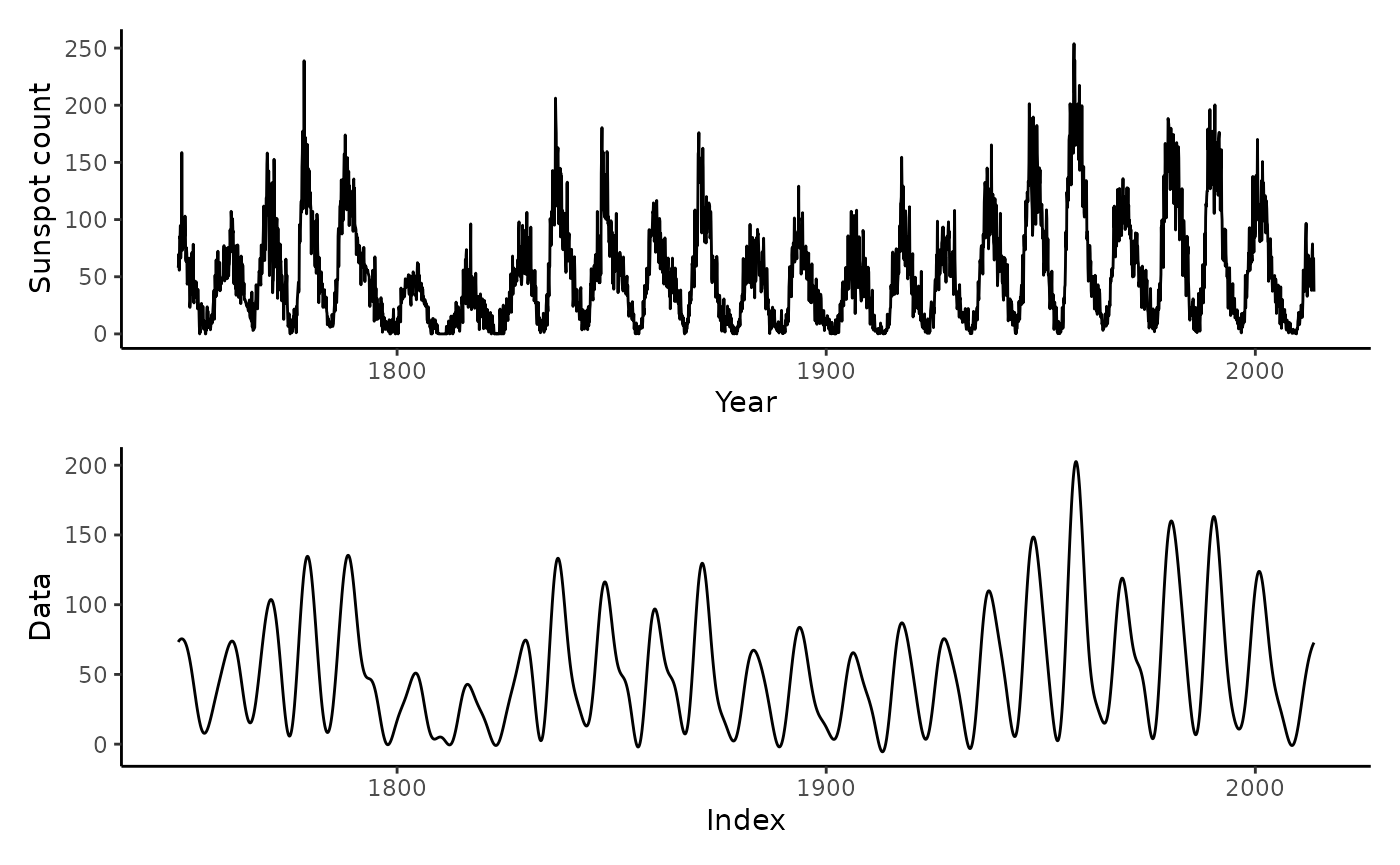
To denoise the sunspot.month data, we suppress high-frequency components:

ggplot(fortify(sunspot.month)) +
  geom_line(aes(x = Index, y = Data)) +
  ylab("Sunspot count") +
  xlab("Year") +
  theme_classic() ->
p1

sunspot.month |>
  fftab() |>
  to_polr() |>
  dplyr::mutate(mod = ifelse(abs(.dim_1) > 0.2, 0, mod)) |>
  ifftab() ->
smoothed

ggplot(fortify(smoothed)) +
  geom_line(aes(x = Index, y = Data)) +
  theme_classic() ->
p2

p1 / p2

The dplyr::mutate call zeros out the magnitudes of any components with periodicity of 5 years or fewer.

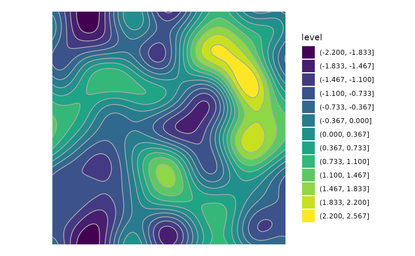
Example 3: 2D Gaussian Autocorrelation

A gaussian kernel in the frequency domain has mangnitudes

$\left \lvert \left ( \vec f \right) \right \rvert \propto e^{-\pi^2\sigma^2 \left \lVert \vec f \right \rVert ^2}$

where $\left \lVert \vec f \right \rVert ^2$ is the sum of squared frequencies across dimensions. fftab provides functions for computing the L2 norm and squared L2 norm of the frequencies in any number of dimensions allowing easy access to these numbers in computations.

sigma <- 64
scale_fac <- -pi^2 * sigma^2

matrix(rnorm(512 * 512), 512) |>
  fftab() |>
  to_polr() |>
  add_l2sq() |>
  dplyr::mutate(mod = mod * exp(scale_fac * l2sq)) |>
  ifftab() ->
gauss_acf

tidyr::expand_grid(x = 1:512, y = 1:512) |>
  tibble::add_column(z = gauss_acf |> as.vector() |> scale()) |>
  ggplot() +
  aes(x = x, y = y, z = z) +
  geom_contour_filled(bins = 16) +
  geom_contour(bins = 16, color = "darkgrey") +
  coord_equal() +
  theme_void()

The result of this operation has the autocorrelation a circular convolution of white-noise and a gaussian kernel.

Conclusion

The fftab package simplifies Fourier Transform operations by combining spectral coefficients and frequencies in a tibble. This integration enables seamless manipulation of frequency-domain data with tidyverse tools, making fftab a powerful resource for spectral analysis.